ENTS,
            On November 1, 2008 , President of ENTS Will Blozan and new Ent from PA Mike Dunn climbed the Jake Swamp white pine in Mohawk Trail State Forest , Charlemont , MA . Will tape drop measured the Jake tree, as we call it, to an impressive height of 168.5 feet, tallest in New England . That height was within 0.1 feet of my most probable ground-based measurement and 0.4 feet of John Knuerr ’s single measurement.

            While descending the Jake tree, Will took 17 circumference measurements at points he chose based on where he saw a change of form. Will’s measurements were taken from a height of 130 feet down to ground-level. The remaining part of Jake, i.e from 130 to 168.5 feet was modeled as a right circular cone. The portion from ground-level to 130 feet was modeled as a series of frustums of right circular cones. Using the formula for a frustum that we’ve often repeated in emails, a volume of 581.9 cubic feet was obtain for the section from base to 130 feet. At a dinner at the Charlemont Inn, Will’s quick calculations produced 573 cubes. I’m unsure of where the discrepancy lies. The remainder of the trunk volume above 130 feet was approximated at 17.2 cubic feet. The total volume of the frustums and final cone equals 599.1 cubes. That is the modeled trunk volume of Jake following the protocol that we’ve previously applied.

            The question arises as to what volume we might derive were we to develop a regression-based model using height above base as the independent variable and radius as the dependent. This question was answered with the help of Minitab 13, a statistical software package. The three models below show the results. The first assumes a linear relationship, the second fits a parabola to the data, and the third fits a cubic equation (3 rd degree polynomial).

             Based on the high degree of fit for the cubic equation, an Excel workbook was developed that reflects all the modeling work. The workbook is provided as the attachment. However, the 3 rd spreadsheet in the workbook can be used as a standalone worksheet. The method used in the spreadsheet is explained after presentation of the models.

Regression Analysis: C2 versus C1 (linear)

The regression equation is

C2 = 1.68 - 0.00802 C1

Predictor        Coef     SE Coef          T        P

Constant      1.68283     0.02591      64.95    0.000

C1         -0.0080216   0.0003677     -21.81    0.000

S = 0.06257     R-Sq = 97.1%     R-Sq(adj) = 96.9%

Analysis of Variance

Source            DF          SS          MS         F        P

Regression         1      1.8628      1.8628    475.87    0.000

Residual Error    14      0.0548      0.0039

Total             15      1.9177

Unusual Observations

Obs         C1         C2         Fit      SE Fit    Residual    St Resid

  1          3     1.8167      1.6628      0.0252      0.1539        2.69R

R denotes an observation with a large standardized residual

Polynomial Regression Analysis: C2 versus C1 (parabola)

The regression equation is                             

C2 = 1.68798 - 0.0083477 C1                            

 + 0.0000027 C1**2                                     

S = 0.0647927      R-Sq = 97.2 %      R-Sq(adj) = 96.7 %

Analysis of Variance

Source            DF         SS         MS         F      P

Regression         2    1.86308   0.931540   221.896  0.000

Error             13    0.05458   0.004198                

Total             15    1.91765                           

Source      DF     Seq SS          F      P

Linear       1    1.86285    475.867  0.000

Quadratic    1    0.00023      0.055  0.819

Polynomial Regression Analysis: C2 versus C1 (cubic)

The regression equation is                             

C2 = 1.73507 - 0.0144310 C1                            

 + 0.0001269 C1**2 - 0.0000006 C1**3                   

S = 0.0582937      R-Sq = 97.9 %      R-Sq(adj) = 97.3 %

Analysis of Variance

Source            DF         SS         MS         F      P

Regression         3    1.87688   0.625626   184.107  0.000

Error             12    0.04078   0.003398                

Total             15    1.91765                           

Source      DF     Seq SS          F      P

Linear       1    1.86285    475.867  0.000

Quadratic    1    0.00023      0.055  0.819

Cubic        1    0.01380      4.060  0.067

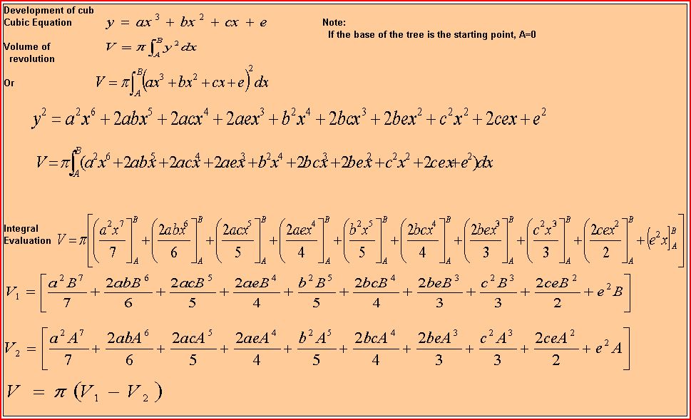
            How does one take any of the above regression models and calculate trunk volume? It is fairly straightforward. All t hese models predict trunk radius at specified heights above the base of the tree (actually from an arbitrary starting at one point on the trunk and going to another). If we plot the graph of the regression equation with radius on the Y axis and height on the X axis, we can then imagine rotating the radius curve around the X axis to generate a three-dimensional image of the trunk. Integral calculus then gives us a method of computing the volume of the generated geometric solid. Spreadsheet 2 (EvalOf Integral) of the attached workbook shows the resul. T he third spreadsheet (CalFinalVol) applies the process to the Jake Tree. The volume derived through the regression cubic model is about 17 cubes larger than the model developed by adding the volumes of the separate frustums. The frustum model is the more accurate.

            I pass by observing that spreadsheet 3  can stand alone. If the user supplies values for the coefficients of the cubic equation and the beginning and ending heights (limits of integration), the spreadsheet calculates the trunk volume automatically. As with all my spreadsheets, the green cells are for user input. The remaining cells are protected. Oh yes, there is also a provision for adding a separate amount such as a conical determination of the top of the tree from the point of highest circumference measurement to the tip. The amount added could just as easily be at the bottom of the tree or a combination of sections. Basically, t he cubic equation can be used to model a section of trunk. Different equations could be developed to model different trunk segments based on w hat the educated eye sees as different areas of curvature that could not be modeled well by one equation .

            Equation derivation requires a regression program to compute the coefficients of the cubic equation. Statistical programs are available, but I plan to develop a spreadsheet version so that the Ents who don’t want to wade through statistical software packages can rely on a single spreadsheet model that only requires the input radial and height measurements, then generates the cubic equation and performs the integration to arrive at trunk volume.

Bob